Browse Bar: Browse by Author | Browse by Category | Browse by Citation | Advanced Search
The Self-Organizing ARTMAP Rule Discovery (SOARD) system derives relationships among recognition classes during online learning. SOARD training on input/output pairs produces direct recognition of individual class labels for new test inputs. As a typical supervised system, it learns many-to-one maps, which recognize different inputs (Spot, Rex) as belonging to one class (dog). As an ARTMAP system, it also learns one-to-many maps, allowing a given input (Spot) to learn a new class (animal) without forgetting its previously learned output (dog), even as it corrects erroneous predictions (cat).
Santiago Olivera
The main code is in SOARD.m. It takes as inputs a labeled dataset for Stage 1 learning, an unlabeled dataset for Stage 2, and a flag to determine if you want to create a new data ordering or work with a previously created one. It requires the following functions: ordenes.m, ppf.m, fabso.m, rigido.m, and soSelfSupLearning. All of them are included in the files.
Windows
Matlab
Public domain software
This software implements the motion pathway of the 3D FORMOTION model.
Jasmin Leveille
How do spatially disjoint and ambiguous local motion signals in multiple directions generate coherent and unambiguous representations of object motion? Various motion percepts, starting with those of Duncker and Johansson, obey a rule of vector decomposition, whereby global motion appears to be subtracted from the true motion path of localized stimulus components. Then objects and their parts are seen moving relative to a common reference frame. A neural model predicts how vector decomposition results from multiple-scale and multiple-depth interactions within and between the form and motion processing streams in V1-V2 and V1-MST, which include form grouping, form-to-motion capture, figure-ground separation, and object motion capture mechanisms. These mechanisms solve the aperture problem, group spatially disjoint moving object parts via illusory contours, and capture object motion direction signals on real and illusory contours. Inter-depth directional inhibition causes a vector decomposition whereby motion directions of a moving frame at a nearer depth suppress these directions at a farther depth and cause a peak shift in the perceived directions of object parts relative to the frame.
The model is implemented in C++. The JAMA/TNT library is used for computation of the singular value decomposition, and FFTW is used for fast convolution of non-separable kernels. The code was developed for Windows 64 bits and comes with a Microsoft Visual Studio Solution File (formotion.sln). Input to the model should be encoded in XML format. A sample input is provided (divita_120_120_7_40_2_M1_0.5_1_1__10_10.xml). A pre-compiled executable is also provided (formotion.exe). Documentation can be generated using DOxygen. The program can be run by typing "formotion.exe -p plist.txt -i inputs.txt -s" at the DOS command line.
PC with Windows 64 bits
C++
Public domain software
CONFIGR-STARS applies CONFIGR (CONtour FIgure and GRound) to solve the problem of star image registration. CONFIGR (CONtour FIgure and GRound) is a computational model based on principles of biological vision that completes sparse and noisy image figures. Star signatures based on CONFIGR connections uniquely identify a location in the sky, with the geometry of each signature encoding and locating unknown test images.
Arun Ravindran
CONFIGR-STARS, a new methodology based on a model of the human visual system, is developed for registration of star images. The algorithm first applies CONFIGR, a neural model that connects sparse and noisy image components. CONFIGR produces a web of connections between stars in a reference starmap or in a test patch of unknown location. CONFIGR-STARS splits the resulting, typically highly connected, web into clusters, or “constellations.” Cluster geometry is encoded as a signature vector that records edge lengths and angles relative to the cluster’s baseline edge. The location of a test patch cluster is identified by comparing its signature to signatures in the codebook of a reference starmap, where cluster locations are known. Simulations demonstrate robust performance in spite of image perturbations and omissions, and across starmaps from different sources and seasons. Further studies would test CONFIGR-STARS and algorithm variations applied to very large starmaps.
3 files are included in the compressed software package:
configr_stars_train.m -- to generate star signatures for the starmap.
configr_stars_test.m -- to locate an unknown patch.
configr_stars_extract_nodes_edges.m -- to extract signatures from CONFIGR conenctions.
NOTE: Please refer to CONFIGR software (http://techlab.bu.edu/resources/software_view/configr_contour_figure_ground/) on how to run CONFIGR
OS independent
Matlab
Retail software
Gail Carpenter
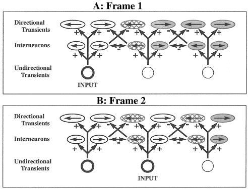
This microcircuit models how direction selectivity appears in the directional transient cells, which are found in layer 4Ca of area V1 for macaques.
Below are links to source article and zipped file that contains a MATLAB-based graphical user interface with additional access to the directional transient cell network equation, description, and source code.
Praveen Pilly
The microcircuit for directional transient network simulates how two cell types interact to realize directional selectivity at a wide range of speeds: directional transient cells, which generate output signals, and directional inhibitory interneurons, which influence these directional output signals (Grossberg et al., 2001). This interaction is consistent with rabbit retinal data concerning how bipolar cells interact with inhibitory starburst amacrine cells and direction-selective ganglion cells, and how starburst cells interact with each other and with ganglion cells (Fried, Münch, & Werblin, 2002). This predicted role of starburst cells in ensuring directional selectivity at a wide range of speeds has not yet been tested. This circuit is used to generate local directional signals in a number of motion processing models (Chey et al., 1997; Grossberg et al., 2001; Berzhanskaya et al., 2007; Grossberg & Pilly, 2008).
To use the software for the directional transient cells, download the package (DTransientCells.zip) from the Download(s) below and unzip the contents into a local folder. Open MATLAB and change the current directory to the folder. At the command prompt, type DTCgui to begin using the software via a graphical user interface.
Any operating system that can support MATLAB
MATLAB
Freeware
Praveen K. Pilly
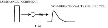
This microcircuit models how ON magnocellular cells in Retina and lateral geniculate nucleus transiently respond to temporal luminance changes in the visual input.
Below are links to source article and zipped file that contains a MATLAB-based graphical user interface with additional access to the non-directional transient cell equation, description, and source code.
Praveen Pilly
The microcircuit for non-directional transient cells simulates how magnocellular cells in Retina and lateral geniculate nucleus are activated in response to temporal changes in the visual stimulus. This acts as the first stage of various motion processing models (Chey et al., 1997; Grossberg et al., 2001; Berzhanskaya et al., 2007; Grossberg & Pilly, 2008). Two kinds of these magnocellular cells, ON and OFF, give transient responses to bright stimulus onset and offset or dark stimulus offset and onset, respectively (Baloch et al., 1999; Schiller, 1992). These transient responses are sensitive to the contrast of the moving dots but not to the duration for which stimulus stays on or off beyond a critical duration (see Figure 2 in Grossberg & Pilly, 2008). ON and OFF transient cells code the leading and trailing edges, respectively, of a moving bright object (Schiller, 1992). Modeling the cross talk between ON and OFF cells is important to simulate direction judgments of contrast polarity-reversing or reverse-phi motion stimuli (Anstis, 1970; Anstis & Rogers, 1975; Baloch et al., 1999; Chubb & Sperling, 1989).
To use the software for the non-directional transient cells, download the package (NDTransientCells.zip) from the Download(s) below and unzip the contents into a local folder. Open MATLAB and change the current directory to the folder. At the command prompt, type NDTCgui to begin using the software via a graphical user interface.
Any operating system that can support MATLAB
MATLAB
Freeware
Praveen K. Pilly, Bret Fortenberry
The code allows for the creation, training, and testing of a Fuzzy ARTMAP neural network system. The following example datasets are also included in the zip file.
Sai Gaddam
A new neural network architecture is introduced for incremental supervised learning of recognition categories and multidimensional maps in response to arbitrary sequences of analog or binary input vectors, which may represent fuzzy or crisp sets of features. The architecture, called fuzzy ARTMAP, achieves a synthesis of fuzzy logic and adaptive resonance theory (ART) neural networks by exploiting a close formal similarity between the computations of fuzzy subsethood and ART category choice, resonance and learning. Fuzzy ARTMAP also realizes a new minimax learning rule that conjointly minimizes predictive error and maximizes code compression, or generalization. This is achieved by a match tracking process that increases the ART vigilance parameter by the minimum amount needed to correct a predictive error. As a result, the system automatically learns a minimal number of recognition categories, or “hidden units,” to meet accuracy criteria. Category proliferation is prevented by normalizing input vectors at a preprocessing stage. A normalization procedure called complement coding leads to a symmetric theory in which the AND operator (∧) and the OR operator (∨) of fuzzy logic play complementary roles. Complement coding uses on cells and off cells to represent the input pattern, and preserves individual feature amplitudes while normalizing the total on cell/off cell vector. Learning is stable because all adaptive weights can only decrease in time. Decreasing weights correspond to increasing sizes of category “boxes.” Smaller vigilance values lead to larger category boxes. Improved prediction is achieved by training the system several times using different orderings on the input set. This voting strategy can also be used to assign confidence estimates to competing predictions given small, noisy, or incomplete training sets. Four classes of simulations illustrate fuzzy ARTMAP performance in relation to benchmark back propagation and genetic algorithm systems. These simulations include (i) finding points inside versus outside a circle; (ii) learning to tell two spirals apart, (iii) incremental approximation of a piecewise-continuous function; and (iv) a letter recognition database. The fuzzy ARTMAP system is also compared with Salzberg’s NGE system and with Simpson’s FMMC system.
A Tutorial is included in the zip file and can be accessed through the GUI's menu.
To execute examples, execute ARTMAPgui at the MATLAB command line. From the GUI menu, select Run tab and select one of the following datasets from the dropdown menu.
To provide your own dataset, execute fuzzyARTMAPTester in the MATLAB command line.
Usage: [a,b,c] = biasedARTMAPTester(dataStruct,lambda_value)
The MATLAB struct dataStruct should have the following format.
The datastruct fields are:
training_input: [f features X m records]
training_output: [m labels X 1]
test_input: [f features X n records]
test_output: [n labels X 1]
description: ‘dataset_title’
descriptionVerbose: ‘A more detailed description of the dataset (optional)’
Any OS that runs Matlab
MATLAB
Freeware
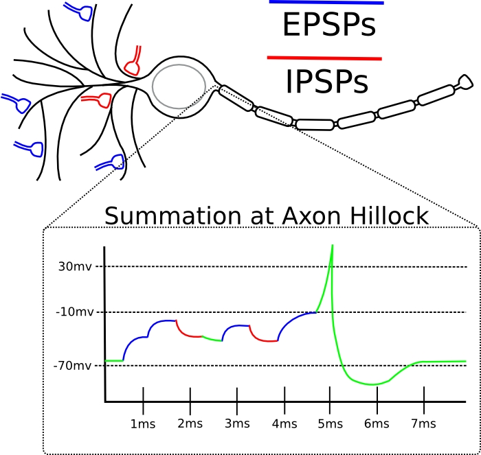
A model to demonstrate the effect of Excitatory Postsynaptic Potentials (EPSP) and Inhibitory Postsynaptic Potentials (IPSP) on a neuron. The model is based on synaptic conductance equations from (Kohn and Worgotter 1998) and a fast resonate-and-fire neuron spiking equation from (Izhikevich 2001).
Izhikevich, EM (2001). Resonate-and-fire neurons. Neural Networks 14: 883-894.
Kohn, J and Worgotter, F (1998). Employing the Z-transform to Optimize the calculation of the synaptic conductance of NMDA and other synaptic channels in network simulations. Neural Computation 10: 1639-1651.
Hodgkin, A. L., & Huxley, A. F. (1952). Quantitative description of membrane current and its application to conduction and excitation in nerve. Journal of Physiology, 117, 500–544.
Bret Fortenberry
A model to show the properties of EPSPs and IPSPs in the postsynaptic cell. The model allows a user to adjust the number of EPSP and IPSP inputs, the rise and fall times and the weighted effect on the postsynaptic cell. The model displays the current of the EPSP and the IPSP and the spiking output of the postsynaptic cell.
An excitatory postsynaptic potentials (EPSP) is a temporary depolarization of postsynaptic membrane caused by the flow of positively charged ions into the postsynaptic cell as a result of opening of ligand-sensitive channels. An EPSP is received when an excitatory presynaptic cell, connected to the dendrite, fires an action potential. The EPSP signal is propagated down the dendrite and is summed with other inputs at the axon hilllock. The EPSP increases the neurons membrane potential. When the membrane potential reaches threshold the cell will produce an action potential and send the information down the axon to communicate with postsynaptic cells. The strength of the EPSP depends on the distance from the soma. The signal degrades across the dendrite such that the more proximal connections have more of an influence.
An inhibitory postsynaptic potentials (IPSP) is a temporary hyperpolarization of postsynaptic membrane caused by the flow of negatively charged ions into the postsynaptic cell. An IPSP is received when an inhibitory presynaptic cell, connected to the dendrite, fires an action potential. The IPSP signal is propagated down the dendrite and is summed with other inputs at the axon hilllock. The IPSP decreases the neurons membrane potential and makes more unlikely for an action potential to occur. A postsynaptic cell typically has less inhibitory connections but the connections are closer to the soma. The proximity of the inhibitory connections produces a stronger signal such that fewer IPSPs are needed to cancel out the effect of EPSPs.
The membrane potential and spiking rate are dependent on a cells biophysical mechanism and the interaction of the cells internal and external voltage. Hodgkin and Huxley (1952) have introduced a standard model to describe the dynamics of cell's membrane potential. That model, described in terms of differential equations, tends to be computationally slow. Over the years, several other simplified spiking models have been designed. Although the later models are faster, they are less accurate than the Hodgkin and Huxley model. In this demonstration the Izhikevich resonate-and-fire model is used. This spiking model is used because it is faster than quadratic firing models and more biologically accurate than integrate and fire models.
A demonstration of the effects of multiple EPSPs and IPSPs on a single neuron. To run the code open download the file epsp_ipsp.zip from the download section at the bottom. Unzip the file and open Matlab. Run epsp_ipsp_gui from the root epsp_ipsp directory.
Linux/Unix, Machintosh, Windows
Matlab
Demo software
Bret Fortenberry, Jasmin Leveille, Massimiliano Versace, Kadin Tseng, Doug Sondak, Jesse Palma, Gail Carpenter
mfc2html is a combination of matlab m-file and Perl script to post a list of m-files in a HTML format for automatic production of HTML documentation in a folder containing MATLAB code.
Kadin Tseng
mfc2html is a combination of matlab m-file and Perl script to post a list of m-files in a HTML format for automatic production of HTML documentation in a folder containing MATLAB code.
mfc2html is a combination of matlab m-file and Perl script to post a list of m-files in a HTML format for easy reading.
Windows, Linux
Perl, matlab
Shareware
An Automated Matlab Graphical User Interface builder. For a quick overview on how to use the builder see the tutorial GUI4GUI_for_Dummies.pdf. For more advanced descriptions, and more features see the official GUI4GUI Users Guide listed below.
Kadin Tseng
An Automated Graphical User Interface builder designed for CNS students and faculty to create a self contained documentation for codes and models developed during their research.
An Automated Graphical User Interface builder that generates a GUI in the form of an .m-file.
Any OS that runs Matlab. (Windows, Mac, Linux)
MATLAB
Shareware
Kadin Tseng, Doug Sondak, Robert Thijs Kozma
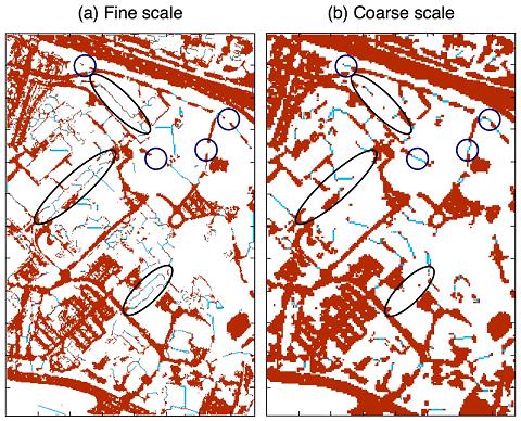
CONFIGR (CONtour FIgure and GRound) is a model that performs long-range contour completion on large-scale images. CONFIGR accomplishes this through a mechanism that fills-in both figure and ground via complementary process.
Sai Gaddam
CONFIGR (CONtour FIgure GRound) is a computational model based on principles of biological vision that completes sparse and noisy image figures. Within an integrated vision/recognition system, CONFIGR posits an initial recognition stage which identifies figure pixels from spatially local input information. The resulting, and typically incomplete, figure is fed back to the “early vision” stage for long-range completion via filling-in. The reconstructed image is then re-presented to the recognition system for global functions such as object recognition. In the CONFIGR algorithm, the smallest independent image unit is the visible pixel, whose size defines a computational spatial scale. Once pixel size is fixed, the entire algorithm is fully determined, with no additional parameter choices. Multi-scale simulations illustrate the vision/recognition system. Open-source CONFIGR code is available online, but all examples can be derived analytically, and the design principles applied at each step are transparent. The model balances filling-in as figure against complementary filling-in as ground, which blocks spurious figure completions. Lobe computations occur on a subpixel spatial scale. Originally designed to fill-in missing contours in an incomplete image such as a dashed line, the same CONFIGR system connects and segments sparse dots, and unifies occluded objects from pieces locally identified as figure in the initial recognition stage. The model self-scales its completion distances, filling-in across gaps of any length, where unimpeded, while limiting connections among dense image-figure pixel groups that already have intrinsic form. Long-range image completion promises to play an important role in adaptive processors that reconstruct images from highly compressed video and still camera images.
Usage:
I_output = runCONFIGR(I,PixRes)
This runs CONFIGR with the following defaults:
PixRes: pixel resolution default=1: CONFIGR pixel resolution is the same as that of the input image
Advanced Options:
I_output = runCONFIGR(I,PixRes,NumIter,ShrinkFact)
I: input image
PixRes: pixel resolution 1: fine 2: medium 3: coarse
The following options provide computational flexibility but are not model parameters.
NumIter: number of iterations CONFIGR simulation can be forced to stop early by setting a low number of iterations.
ShrinkFact: ratio of desired image size to actual size Sparse images can be resized for faster runtimes.
Raw CONFIGR output (ground and figure-filled rectangles, and interpolating diagonals)
can be obtained using [I_output, I_output_raw, Idiagonals]=runCONFIGR(I)
Simple cell and complex cell activations are computed in CONFIGR_6_FindBound.mImage: Select a rectangular image.
Lobe propagation is computed in: CONFIGR_6_LobePropagate.m
Empty Rectangles are computed in: EmptyRectangleTypeOne_Ground_6.m, EmptyRectangleTypeTwo_Ground_6.m
Relevant File: FillingGROUND.mAn empty rectangle is eligible for filling-in as ground if it contains an empty ground corner or if it shares an edge with one or more filled-ground pixels.
Relabel wall corners that have become empty figure or empty ground. For each such corner, add newly created empty rectangles to the marked list. Relabel as filled-ground the pixels of each newly created empty rectangle of size equal to or smaller than the current loop size, if the rectangle is eligible for filling-in as ground. Relabel newly filled corners. Remove from the list of marked rectangles all that are no longer empty, because they intersect newly filled rectangles.Iterate corner and rectangle updates until no more changes occur.
Relevant File: FillingFIGURE.mLoop from smallest to largest empty rectangle (filling-in as figure) {
After all rectangles of the loop size have been filled as figure, relabel affected corners. Some empty corners that had previously been wall may now be empty figure or empty ground corners. For each such corner, add newly created empty rectangles to the marked list. Fill as ground newly created marked rectangles, if the rectangle contains an empty ground corner or is adjacent to one or more filled ground pixels. Remove from the list of marked rectangles all that are no longer empty, because they intersect newly filled rectangles.Iterate corner and rectangle updates until no more changes occur.
Fill as figure each remaining newly created marked rectangle of size equal to or smaller than the current loop size.
Remove from the list of marked rectangles all that are no longer empty, because they intersect newly filled rectangles.
Any
MATLAB
Public domain software
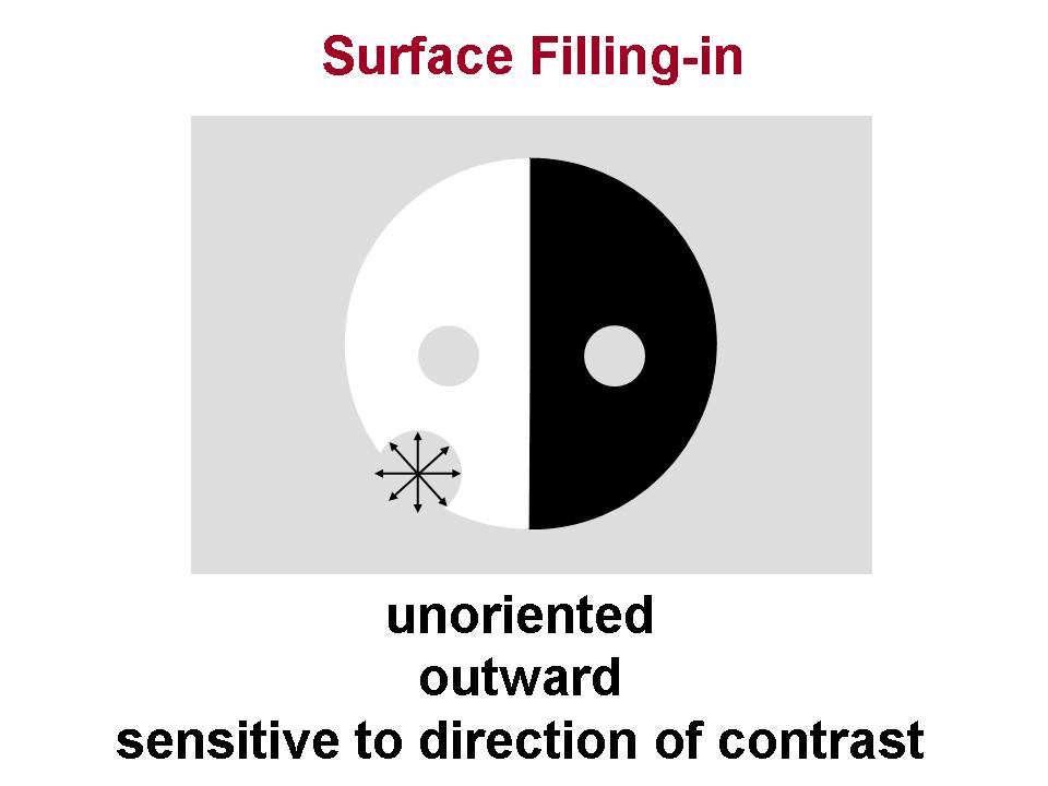
Filling-in GUI microassembly. The package contains a MATLAB implementation of diffusive filing-in model. The demo simulation is based on Craik-O'Brien-Cornsweet Effect(COCE). The package provides GUI interface to control luminance of COCE stimulus components which have impact on the model's output. The software can be run from matlab command line by typing Filling_in at the prompt. Necessary documentation as well as source code is provided.
Gennady Livitz
Present implementation of diffusive filling-in model demonstrates dynamics of neural signal spreading on the example of Craik-O'Brien-Cornsweet Effect. Filling-in process is implemented as a set of non-linear differential equations that control spreading of the activity of the Feature Contour System signals (brightness, color) within the image segments defined by the Boundary Contour System signals. The demo example simulates 1D filling-in process and allows the user to see the impact of luminance contrast in the COCE configuration on the output of the present implementation of diffusive filling-in model.
Filing-in GUI microassembly. Unzip archive. Run by typing Filling-in at MATLAB prompt
No dependency
MATLAB
Public domain software
Gennady Livitz, Gail Carpinter, Pilly Praveen, Massimiliano Versace
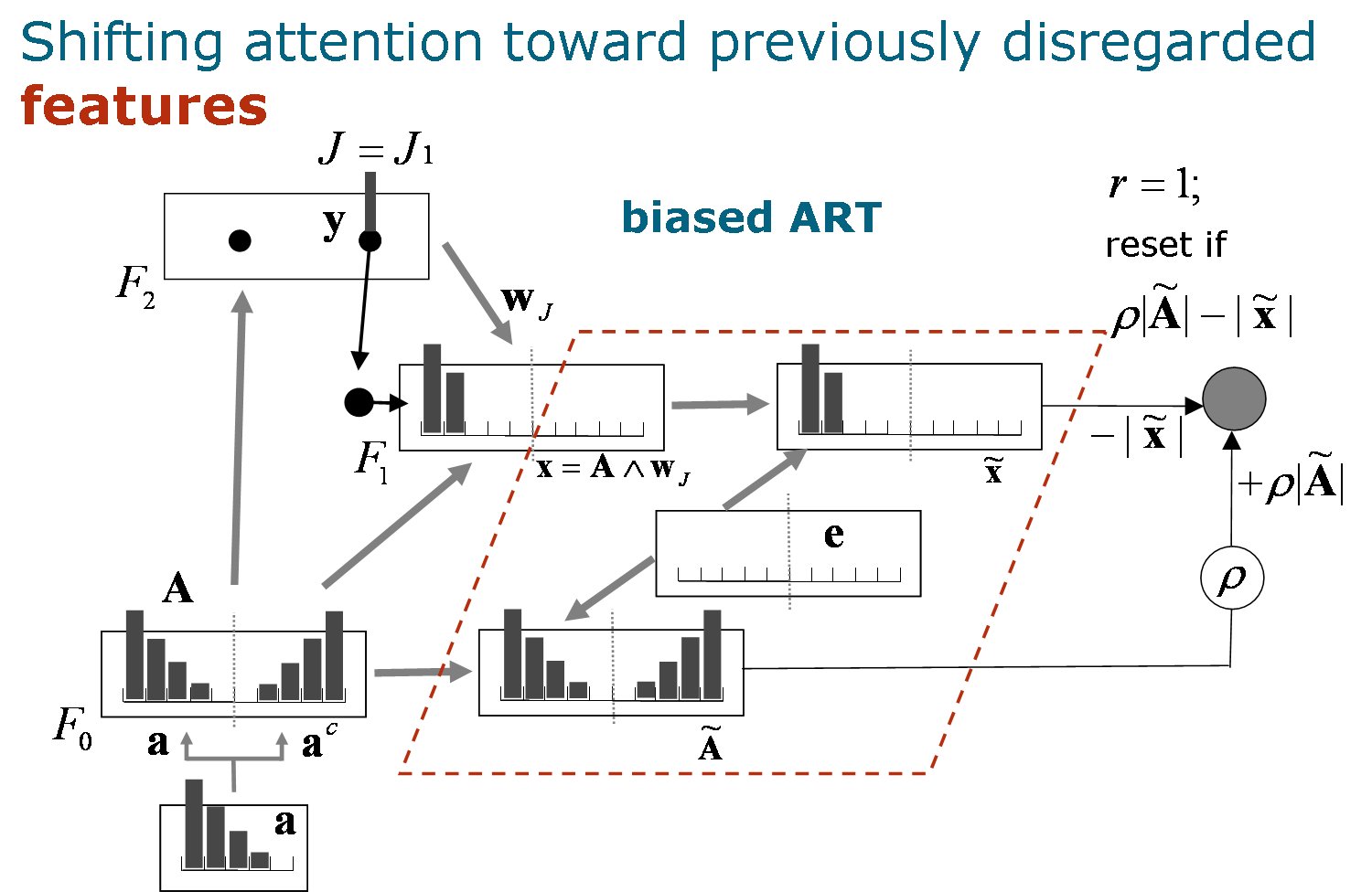
Memories in Adaptive Resonance Theory (ART) networks are based on matched patterns that focus attention on those portions of bottom-up inputs that match active top-down expectations. While this learning strategy has proved successful for both brain models and applications, computational examples show that attention to early critical features may later distort memory representations during online fast learning. For supervised learning, biased ARTMAP (bARTMAP) solves the problem of over-emphasis on early critical features by directing attention away from previously attended features after the system makes a predictive error. Small-scale, hand-computed analog and binary examples illustrate key model dynamics. Two-dimensional simulation examples demonstrate the evolution of bARTMAP
memories as they are learned online. Benchmark simulations show that featural biasing also improves performance on large-scale examples. One example, which predicts movie genres and is based, in part, on the Netflix Prize database, was developed for this project. Both first principles and consistent performance improvements on all simulation studies suggest that featural biasing should be incorporated by default in all ARTMAP systems. Benchmark datasets and bARTMAP code are available here.
Disclaimer
This software is provided free of charge. As such, the authors assume no responsibility for the programs' behavior. While they have been tested and used in-house for three years, no claim is made that biased ARTMAP implementations are correct or bug-free. They are used and provided solely for research and educational purposes. No liability, financial or otherwise, is assumed regarding any application of biased ARTMAP.
Feedback
Have questions? Found a bug? Please send comments to: gsc@cns.bu.edu
Sai Gaddam
Memories in Adaptive Resonance Theory (ART) networks are based on matched patterns that focus attention on those portions of bottom-up inputs that match active top-down expectations. While this learning strategy has proved successful for both brain models and applications, computational examples show that attention to early critical features may later distort memory representations during online fast learning. For supervised learning, biased ARTMAP (bARTMAP) solves the problem of over-emphasis on early critical features by directing attention away from previously attended features after the system makes a predictive error. Small-scale, hand-computed analog and binary examples illustrate key model dynamics. Two-dimensional simulation examples demonstrate the evolution of bARTMAP memories as they are learned online. Benchmark simulations show that featural biasing also improves performance on large-scale examples. One example, which predicts movie genres and is based, in part, on the Netflix Prize database, was developed for this project. Both first principles and consistent performance improvements on all simulation studies suggest that featural biasing should be incorporated by default in all ARTMAP systems.
This description is also available in the ReadMe.txt file provided in the downloadable zipped folder.
The following examples can be run by executing biasedARTMAP_examples.m:
Any
MATLAB
Public domain software
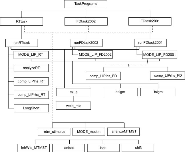
MOtion DEcision (MODE) model is a neural model of perceptual decision-making that discriminates the direction of an ambiguous motion stimulus and simulates behavioral and physiological data obtained from macaques performing motion discrimination tasks.
Praveen Pilly
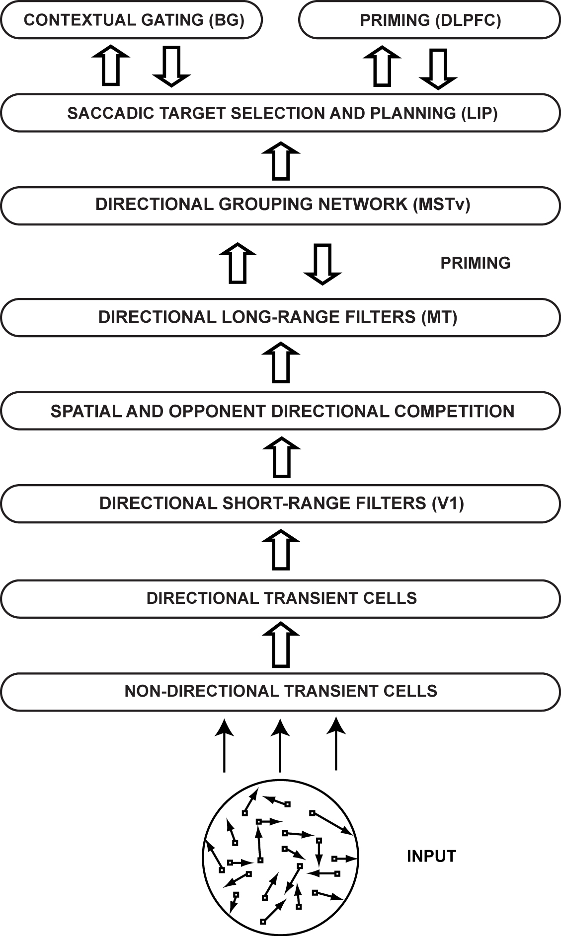
How does the brain make perceptual decisions? Speed and accuracy of saccadic decisions regarding motion direction depend on the inherent ambiguity in the motion stimulus and correlate with the temporal dynamics of firing rates in parietal and frontal cortical neurons of macaque monkeys. The MOtion DEcision (MODE) model incorporates interactions within and between Retina/lateral geniculate nucleus, primary visual cortex, middle temporal area, medial superior temporal area, and lateral intraparietal area, gated by basal ganglia, to provide a functional and mechanistic understanding of motion-based decision-making behavior in response to the experimental motion stimuli. The model demonstrate how motion capture circuits in middle temporal and medial superior temporal areas gradually solve the informational aperture problem, while interacting with a noisy recurrent competitive field in lateral intraparietal area whose self-normalizing choice properties make probabilistic directional decisions in real time. Quantitative model simulations include the time course of lateral intraparietal neuronal dynamics, as well as behavioral accuracy and reaction time properties, during both correct and error trials at different levels of input ambiguity in both fixed duration and reaction time tasks.
[ http://techlab.bu.edu/resources/data_view/mode_model_demos/ ] The demos show precomputed temporal dynamics at each MODE model stage with a brief description for three distinct input ambiguity (low, medium, and high) cases to provide an insight into the functional roles of the various stages.
[ http://techlab.bu.edu/MODE/Tutorial.pps ] The tutorial provides the motivation behind the MODE model and shows how it works to mechanistically explain the various behavioral and physiological motion decision-making data.
To use the software for the MODE model, download the package (MODE_GUI_070109.zip) from the Download(s) below and unzip the contents into a local folder. Open MATLAB (see Programming Language requirement below) and change the current directory to the folder. Also, set the path to include all the subfolders. At the command prompt, type MODEgui to begin using the software via a GUI (highly recommended). Also, the GUI provides one-stop easy access to model equations and descriptions, relevant articles, tutorial, animated demos, and source code. If you like a more hands-on approach, you can run the MODE model directly by using the main function runTask(.m). The folder includes a detailed READ ME file in \SRC, which is also available in Download(s) on this page.
Any operating system that can support MATLAB.
The software has been tested using MATLAB 7 (32 bit) and MATLAB R2008a (64 bit). Newer versions of MATLAB should work fine.
Freeware
Praveen K. Pilly, Stephen Grossberg, Gail Carpenter, Sai Gaddam, Doug Sondak, Kadin Tseng, Max Versace
Self-Supervised ARTMAP learns about novel features from unlabeled patterns without destroying partial knowledge previously acquired from labeled patterns.
Greg Amis
Computational models of learning typically train on labeled input patterns (supervised learning), unlabeled input patterns (unsupervised learning), or a combination of the two (semisupervised learning). In each case input patterns have a fixed number of features throughout training and testing. Human and machine learning contexts present additional opportunities for expanding incomplete knowledge from formal training, via self-directed learning that incorporates features not previously experienced. This article defines a new self-supervised learning paradigm to address these richer learning contexts, introducing a new neural network called self-supervised ARTMAP. Self-supervised learning integrates knowledge from a teacher (labeled patterns with some features), knowledge from the environment (unlabeled patterns with more features), and knowledge from internal model activation (self-labeled patterns). Selfsupervised ARTMAP learns about novel features from unlabeled patterns without destroying partial knowledge previously acquired from labeled patterns. A category selection function bases system predictions on known features, and distributed network activation scales unlabeled learning to prediction confidence. Slow distributed learning on unlabeled patterns focuses on novel features and confident predictions, defining classification boundaries that were ambiguous in the labeled patterns. Self-supervised ARTMAP improves test accuracy on illustrative lowdimensional problems and on high-dimensional benchmarks. Model code and benchmark data are available from: http://cns.bu.edu/techlab/SSART/.
Demo of medical diagnosis illustration
Java implementation with MATLAB scripts (ZIP)
It was tested using Windows XP SP3 (32-bit), and it should work for other versions and operating systems.
MATLAB 7.3.0 (R2006b) or newer - It was tested using MATLAB 7.3.0 (R2006b)
Public domain software
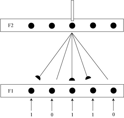
Outstar learning law (Grossberg, 1976) governs the dynamics of feedback connection weights in a standard competitive neural network in an unsupervised manner. This learning models how a neuron can learn a top-down template corresponding to, i.e., expect, a particular input pattern.
Below are links to source article, tutorial, and zipped file that contains a MATLAB-based graphical user interface with additional access to the outstar learning law equation, description, and source code.
Praveen Pilly
The microcircuit for the outstar learning law shows how the dynamics of feedback weights from nodes in a coding field to nodes in an input field are governed within a standard competitive neural network in an unsupervised manner (Grossberg, 1976). This learning models how a neuron in the brain can learn a top-down template corresponding to a particular input pattern. An example simulation allows the users to see how the outstar learning law (Grossberg, 1976) changes weights of connections from the winning node at a coding field that diverge onto an input field. With outstar learning, these efferent weights eventually learn to expect the input activation pattern. This law incorporates Hebbian learning and pre-synaptically gated decay. Typically, learning occurs only for weights that diverge from active nodes in the coding field. However, learning can be further confined to weights projecting away from the most active node in the coding field assuming winner-taking-all coding in the network. This is called competitive learning.
[ http://techlab.bu.edu/MODE/outstar_tutorial.ppt ] The tutorial is a self-contained power point presentation that introduces the outstar learning law.
To use the software for the outstar learning law, download the package (Outstar_GUI_070109.zip) from the Download(s) below and unzip the contents into a local folder. Open MATLAB and change the current directory to the folder. At the command prompt, type outstargui to begin using the software via a GUI.
Any operating system that can support MATLAB
MATLAB
Freeware
Praveen K. Pilly
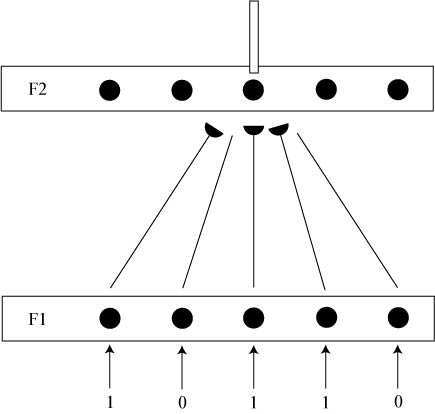
Instar learning law (Grossberg, 1976) governs the dynamics of feedforward connection weights in a standard competitive neural network in an unsupervised manner. This learning models how a neuron can become selectively responsive, or tuned, to a particular input pattern, i.e., a feature detector.
Below are links to source article, tutorial, and zipped file that contains a MATLAB-based graphical user interface with additional access to the instar learning law equation, description, and source code.
Praveen Pilly
The microcircuit for instar learning law shows how the dynamics of feedforward connection weights are governed in a standard competitive neural network in an unsupervised manner. This learning models how a neuron can become selectively responsive, or tuned, to a particular input pattern, i.e., a feature detector. An example simulation allows users to see how afferent weights to a node in the coding field can eventually become similar to the input activation pattern; i.e., they can track the input features over time. This law incorporates Hebbian learning and post-synaptically gated decay. Typically learning occurs only for weights that converge on active nodes in the coding field. However, learning can be further confined to weights projecting to the most active node in the coding field assuming winner-taking-all coding in the network in order to promote stable memories. This is called competitive learning.
[ http://techlab.bu.edu/MODE/instar_tutorial.ppt ] The tutorial is a self-contained power point presentation that introduces the instar learning law.
To use the software for the instar learning law, download the package (Instar_GUI_070109.zip) from the Download(s) below and unzip the contents into a local folder. Open MATLAB and change the current directory to the folder. At the command prompt, type instargui to begin using the software via a graphical user interface.
Any operating system that can support MATLAB
MATLAB
Freeware
Praveen K. Pilly
This is a one-dimensional stand-alone implementation of the Grossberg and Todorović model of a cortical simple cell. The attached zip file contains Matlab code for the model, as well as documentation and a demonstration GUI designed to illustrate the key computational properties. Note that the source for this model is (Grossberg and Todorović, 1988), but only the section pertaining to cortical simple cells is included.
Ben Chandler
This Matlab implementation includes stand-alone source code, simplecell.m, as well as documentation and a GUI-based example. For stand-alone use instructions, see how_to_run.pdf. Otherwise, run main_gui from Matlab to see the full GUI example.
Platform Independent
Matlab
Freeware
Ben Chandler, Gail Carpenter, Praveen K. Pilly, Chaitanya Sai, Doug Sondak, Kadin Tseng, Max Versace
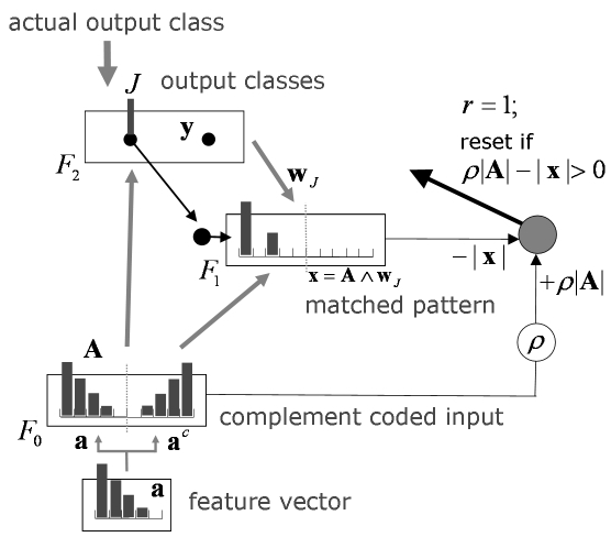
Complement Coding takes as input a vector of feature values, each with an associated lower and upper limit used for normalization. It normalizes each feature value and calculates its complement.
Sai Gaddam
Adaptive Resonance Theory (ART) and ARTMAP networks employ a preprocessing step called complement coding, which models the nervous system’s ubiquitous computational design known as opponent processing (Hurvich & Jameson, 1957). Balancing an entity against its opponent, as in agonist-antagonist muscle pairs, allows a system to act upon relative quantities, even as absolute magnitudes may vary unpredictably. In ART systems, complement coding (Carpenter, Grossberg, & Rosen, 1991) is analogous to retinal ON-cells and OFF-cells (Schiller, 1982). When the learning system is presented with a set of feature values, complement coding doubles the number of input components, presenting to the network both the original feature vector a and its complement.
The complement.zip file contains the Complement Coding Matlab code plus associated documentation and GUI files. To run the code, unzip the files, run Matlab, and type "compgui" at the Matlab prompt.
linux, Windows
Matlab
Public domain software
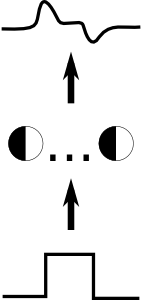
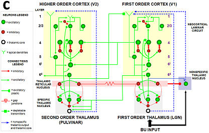
This entry contains the software, implemented in the KDE Integrated NeuroSimulation Software (KInNeSS ) that simulates the Synchronous Matching Adaptive Resonance Theory. SMART was first described in Grossberg and Versace (2008): Spikes, synchrony, and attentive learning by laminar thalamo-cortical circuits.
Max Versace
This article develops the Synchronous Matching Adaptive Resonance Theory (SMART) neural model to explain how the brain may coordinate multiple levels of thalamocortical and corticocortical processing to rapidly learn, and stably remember, important information about a changing world. The model clarifies how bottom-up and top-down processes work together to realize this goal, notably how processes of learning, expectation, attention, resonance, and synchrony are coordinated. The model hereby clarifies, for the first time, how the following levels of brain organization coexist to realize cognitive processing properties that regulate fast learning and stable memory of brain representations: single cell properties, such as spiking dynamics, spike-timing-dependent plasticity (STDP), and acetylcholine modulation; detailed laminar thalamic and cortical circuit designs and their interactions; aggregate cell recordings, such as current source densities and local field potentials; and single-cell and large-scale inter-areal oscillations in the gamma and beta frequency domains. In particular, the model predicts how laminar circuits of multiple cortical areas interact with primary and higher-order specific thalamic nuclei and nonspecific thalamic nuclei to carry out attentive visual learning and information processing. The model simulates how synchronization of neuronal spiking occurs within and across brain regions, and triggers STDP. Matches between bottom-up adaptively filtered input patterns and learned top-down expectations cause gamma oscillations that support attention, resonance, learning, and consciousness. Mismatches inhibit learning while causing beta oscillations during reset and hypothesis testing operations that are initiated in the deeper cortical layers. The generality of learned recognition codes is controlled by a vigilance process mediated by acetylcholine.
This archive contains the NeurlML network, the XML and PNG stimuli and a readme file for simulating the SMART network dynamics.
In order to run the network, download and install KiNneSS from http://www.kinness.net
Linux KDE
C++, NeuroML, XML
Public domain software
KInNeSS is an open source neural simulation software package that allows to design, simulate and analyze the behavior of networks of hundreds to thousands of branched multi-compartmental neurons with biophysical properties such as membrane potential, voltage-gated and ligand-gated channels, the presence of gap junctions or ionic diffusion, neuromodulation channel gating, the mechanism for habituative or depressive synapses, axonal delays, and synaptic plasticity. KInNeSS also allows the output of neurons to control the behavior of a simulated agent.
Anatoli Gorchetchnikov
Making use of very detailed neurophysiological, anatomical, and behavioral data to build biologically-realistic computational models of animal behavior is often a difficult task. Until recently, many software packages have tried to resolve this mismatched granularity with different approaches. This paper presents KInNeSS, the KDE Integrated NeuroSimulation Software environment, as an alternative solution to bridge the gap between data and model behavior. This open source neural simulation software package provides an expandable framework incorporating features such as ease of use, scalability, an XML based schema, and multiple levels of granularity within a modern object oriented programming design. KInNeSS is best suited to simulate networks of hundreds to thousands of branched multi-compartmental neurons with biophysical properties such as membrane potential, voltage-gated and ligand-gated channels, the presence of gap junctions or ionic diffusion, neuromodulation channel gating, the mechanism for habituative or depressive synapses, axonal delays, and synaptic plasticity. KInNeSS outputs include compartment membrane voltage, spikes, local-field potentials, and current source densities, as well as visualization of the behavior of a simulated agent. An explanation of the modeling philosophy and plug-in development is also presented. Further development of KInNeSS is ongoing with the ultimate goal of creating a modular framework that will help researchers across different disciplines to effectively collaborate using a modern neural simulation platform.
KInNeSS Release candidate for 0.3.4.
For updates, please keep checking http://www.kinness.net
Linux. Preferred distribution: KDE
C++
Public domain software